Singular Value Decomposition (SVD)

📌 sklearn.decomposition and SVD

The sklearn.decomposition module provides dimensionality reduction tools such as PCA and TruncatedSVD, both based on Singular Value Decomposition (SVD) ✨.

• 📊 PCA uses SVD to extract principal components after mean-centering the data.
• 🧠 TruncatedSVD applies SVD without mean-centering, making it suitable for sparse data and text analysis (e.g., Latent Semantic Analysis).

🛠️ Applications

SVD is widely used in:

• 📉 Dimensionality reduction
• 🔇 Noise filtering
• 🖼️ Image compression
• 📦 Data compression

---

🔍 SVD – Singular Value Decomposition

SVD is a powerful matrix factorization technique that decomposes a matrix A into three components:

🧮 SVD Decomposition and Formula

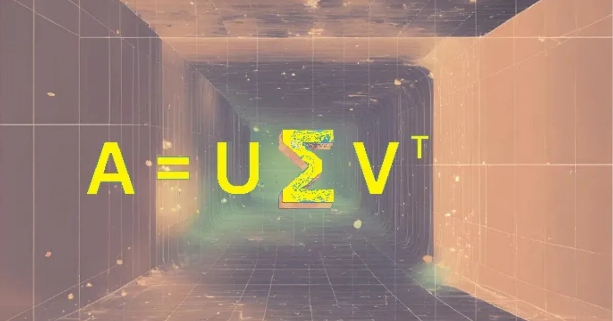
1. A = U Σ Vᵀ
2. U and V are orthogonal matrices:
   • Uᵀ U = I
   • Vᵀ V = I
3. Σ is a diagonal matrix with non-negative singular values σᵢ, sorted in descending order.

Where the dim:

• A is an m x n matrix
• Σ is an m x n diagonal matrix with singular values σᵢ
• U is an m x m matrix of left singular vectors
• Vᵀ is an n x n matrix of right singular vectors

Explicit Matrix Representation

\(\begin{bmatrix}a_{11} & a_{12} & \dots & a_{1n} \\a_{21} & a_{22} & \dots & a_{2n} \\\vdots & \vdots & \ddots & \vdots \\a_{m1} & a_{m2} & \dots & a_{mn}\end{bmatrix}=\begin{bmatrix}\mathbf{u_1} \\\mathbf{u_2} \\\vdots \\\mathbf{u_m}\end{bmatrix}\cdot\begin{bmatrix}\sigma_1 & 0 & \dots & 0 \\0 & \sigma_2 & \dots & 0 \\\vdots & \vdots & \ddots & \vdots \\0 & 0 & \dots & \sigma_r \\0 & 0 & \dots & 0 \\\vdots & \vdots & \ddots & \vdots \\0 & 0 & \dots & 0\end{bmatrix}\cdot\begin{bmatrix}\mathbf{v_1^T} & \mathbf{v_2^T} & \dots & \mathbf{v_n^T}\end{bmatrix}\)

---

🔹 SVD Properties

• The rank of A equals the number of non-zero singular values.
• The first few singular values capture most of the variance.
• Enables low-rank approximation to simplify complex data.

---

🔹 Practical Applications

✔ Dimensionality Reduction (PCA)
✔ Noise Reduction
✔ Recommender Systems
✔ Image Compression
✔ Latent Semantic Analysis (LSA) in NLP

---

🧪 Example: SVD with NumPy

import numpy as np

A = np.array([[0, 0.25, 0],
              [-2, 0, 0]])

u, s, vt = np.linalg.svd(A)

# Convert singular values into matrix form
sigma = np.zeros_like(A, dtype=float)
np.fill_diagonal(sigma, s)

# Print U, Σ, and Vᵀ
for row_u, row_s, row_v in zip(u.tolist(), sigma.tolist(), vt.T.tolist()):
    print(str(row_u).ljust(20), str(row_s).ljust(20), str(row_v))

⚠️ Important:

• np.linalg.svd() returns Σ (singular values) as a 1D vector, not a diagonal matrix.
• To reconstruct the original matrix, you need to convert Σ into a diagonal matrix of appropriate shape.

  # convert Σ (s) to a matrix with the correct shape.
  sigma = np.zeros_like(A, dtype=float)
  np.fill_diagonal(sigma, s)
  

🔄 Low-Rank Approximation with SVD

A = np.array([[2, 1],
              [4, 3],
              [0, -2],
              [-2, -6]])

U, S, VT = np.linalg.svd(A)
k = 1  # number of components
Sigma_k = np.zeros((U.shape[0], VT.shape[0]))
np.fill_diagonal(Sigma_k, S[:k])

A_approx = U[:, :k] @ Sigma_k[:k, :k] @ VT[:k, :]
avg_A_sum = sum(A) / A.shape[0]
A_approx += avg_A_sum

📈 Compare with Linear Regression

We will notice that the methods lead to different approximations because they are based on different error minimization strategies.

• Linear Regression minimizes the squared distance between the data points and the regression line, essentially finding the k-dimensional hyperplane that minimizes the squared distance to the data points along the (k+1)-st dimension.
• SVD, on the other hand, minimizes the squared distance from the points to the plane defined by the most significant singular vectors. It captures the best fit in a lower-dimensional subspace, thus approximating the data.

For more details, you can read wolfram Least Squares Fitting on the difference between SVD and Linear Regression.

🧾 My Jupyter Notebook